When a system has only one solution. Solving systems of linear equations

As is clear from Cramer's theorem, when solving the system linear equations Three cases may occur:

First case: a system of linear equations has a unique solution

(the system is consistent and definite)

Second case: a system of linear equations has an infinite number of solutions

(the system is consistent and uncertain)

** ,

those. the coefficients of the unknowns and the free terms are proportional.

Third case: the system of linear equations has no solutions

(the system is inconsistent)

So the system m linear equations with n called variables non-joint, if she does not have a single solution, and joint, if it has at least one solution. A simultaneous system of equations that has only one solution is called certain, and more than one – uncertain.

Examples of solving systems of linear equations using the Cramer method

Let the system be given

.

Based on Cramer's theorem

………….
,

Where
-

system determinant. We obtain the remaining determinants by replacing the column with the coefficients of the corresponding variable (unknown) with free terms:

Example 2.

.

Therefore, the system is definite. To find its solution, we calculate the determinants

Using Cramer's formulas we find:

So, (1; 0; -1) is the only solution to the system.

To check the solutions to the systems of equations 3 X 3 and 4 X 4, you can use an online calculator using Cramer's solving method.

If in a system of linear equations there are no variables in one or more equations, then in the determinant the corresponding elements are equal to zero! This is the next example.

Example 3. Solve a system of linear equations using the Cramer method:

.

Solution. We find the determinant of the system:

Look carefully at the system of equations and at the determinant of the system and repeat the answer to the question in which cases one or more elements of the determinant are equal to zero. So, the determinant is not equal to zero, therefore the system is definite. To find its solution, we calculate the determinants for the unknowns

Using Cramer's formulas we find:

So, the solution to the system is (2; -1; 1).

6. General system of linear algebraic equations. Gauss method.

As we remember, Cramer's rule and the matrix method are unsuitable in cases where the system has infinitely many solutions or is inconsistent. Gauss method – the most powerful and versatile tool for finding solutions to any system of linear equations, which in every case will lead us to the answer! The method algorithm itself works the same in all three cases. If the Cramer and matrix methods require knowledge of determinants, then to apply the Gauss method you only need knowledge of arithmetic operations, which makes it accessible even to schoolchildren primary classes.

First, let's systematize a little knowledge about systems of linear equations. A system of linear equations can:

1) Have a unique solution.
2) Have infinitely many solutions.
3) Have no solutions (be non-joint).

The Gauss method is the most powerful and universal tool for finding a solution any systems of linear equations. As we remember, Cramer's rule and matrix method are unsuitable in cases where the system has infinitely many solutions or is inconsistent. And the method of sequential elimination of unknowns Anyway will lead us to the answer! In this lesson, we will again consider the Gauss method for case No. 1 (the only solution to the system), the article is devoted to the situations of points No. 2-3. I note that the algorithm of the method itself works the same in all three cases.

Let's go back to the simplest system from class How to solve a system of linear equations?
and solve it using the Gaussian method.

The first step is to write down extended system matrix:
. I think everyone can see by what principle the coefficients are written. The vertical line inside the matrix does not have any mathematical meaning - it is simply a strikethrough for ease of design.

Reference:I recommend you remember terms linear algebra. System Matrix is a matrix composed only of coefficients for unknowns, in this example the matrix of the system: . Extended System Matrix– this is the same matrix of the system plus a column of free terms, in this case: . For brevity, any of the matrices can be simply called a matrix.

After the extended system matrix is ​​written, it is necessary to perform some actions with it, which are also called elementary transformations.

The following elementary transformations exist:

1) Strings matrices can be rearranged in some places. For example, in the matrix under consideration, you can painlessly rearrange the first and second rows:

2) If there are (or have appeared) proportional (as a special case - identical) rows in the matrix, then you should delete All these rows are from the matrix except one. Consider, for example, the matrix . In this matrix, the last three rows are proportional, so it is enough to leave only one of them: .

3) If a zero row appears in the matrix during transformations, then it should also be delete. I won’t draw, of course, the zero line is the line in which all zeros.

4) The matrix row can be multiply (divide) to any number non-zero. Consider, for example, the matrix . Here it is advisable to divide the first line by –3, and multiply the second line by 2: . This action is very useful because it simplifies further transformations of the matrix.

5) This transformation causes the most difficulties, but in fact there is nothing complicated either. To a row of a matrix you can add another string multiplied by a number, different from zero. Let's look at our matrix from a practical example: . First I'll describe the transformation in great detail. Multiply the first line by –2: , And to the second line we add the first line multiplied by –2: . Now the first line can be divided “back” by –2: . As you can see, the line that is ADDED LI – hasn't changed. Always the line TO WHICH IS ADDED changes UT.

In practice, of course, they don’t write it in such detail, but write it briefly:

Once again: to the second line added the first line multiplied by –2. A line is usually multiplied orally or on a draft, with the mental calculation process going something like this:

“I rewrite the matrix and rewrite the first line: »

“First column. At the bottom I need to get zero. Therefore, I multiply the one at the top by –2: , and add the first one to the second line: 2 + (–2) = 0. I write the result in the second line: »

“Now the second column. At the top, I multiply -1 by -2: . I add the first to the second line: 1 + 2 = 3. I write the result in the second line: »

“And the third column. At the top I multiply -5 by -2: . I add the first to the second line: –7 + 10 = 3. I write the result in the second line: »

Please carefully understand this example and understand the sequential calculation algorithm, if you understand this, then the Gaussian method is practically in your pocket. But, of course, we will still work on this transformation.

Elementary transformations do not change the solution of the system of equations

! ATTENTION: considered manipulations can not use, if you are offered a task where the matrices are given “by themselves.” For example, with “classical” operations with matrices Under no circumstances should you rearrange anything inside the matrices!

Let's return to our system. It is practically taken to pieces.

Let us write down the extended matrix of the system and, using elementary transformations, reduce it to stepped view:

(1) The first line was added to the second line, multiplied by –2. And again: why do we multiply the first line by –2? In order to get zero at the bottom, which means getting rid of one variable in the second line.

(2) Divide the second line by 3.

The purpose of elementary transformations – reduce the matrix to stepwise form: . In the design of the task, they just mark out the “stairs” with a simple pencil, and also circle the numbers that are located on the “steps”. The term “stepped view” itself is not entirely theoretical, in scientific and educational literature it is often called trapezoidal view or triangular view.

As a result of elementary transformations, we obtained equivalent original system of equations:

Now the system needs to be “unwinded” in the opposite direction - from bottom to top, this process is called inverse of the Gaussian method.

In the lower equation we already have a ready-made result: .

Let's consider the first equation of the system and substitute the already known value of “y” into it:

Let's consider the most common situation, when the Gaussian method requires solving a system of three linear equations with three unknowns.

Example 1

Solve the system of equations using the Gauss method:

Let's write the extended matrix of the system:

Now I will immediately draw the result that we will come to during the solution:

And I repeat, our goal is to bring the matrix to a stepwise form using elementary transformations. Where to start?

First, look at the top left number:

Should almost always be here unit. Generally speaking, –1 (and sometimes other numbers) will do, but somehow it has traditionally happened that one is usually placed there. How to organize a unit? We look at the first column - we have a finished unit! Transformation one: swap the first and third lines:

Now the first line will remain unchanged until the end of the solution. Now fine.

The unit in the top left corner is organized. Now you need to get zeros in these places:

We get zeros using a “difficult” transformation. First we deal with the second line (2, –1, 3, 13). What needs to be done to get zero in the first position? Need to to the second line add the first line multiplied by –2. Mentally or on a draft, multiply the first line by –2: (–2, –4, 2, –18). And we consistently carry out (again mentally or on a draft) addition, to the second line we add the first line, already multiplied by –2:

We write the result in the second line:

We deal with the third line in the same way (3, 2, –5, –1). To get a zero in the first position, you need to the third line add the first line multiplied by –3. Mentally or on a draft, multiply the first line by –3: (–3, –6, 3, –27). AND to the third line we add the first line multiplied by –3:

We write the result in the third line:

In practice, these actions are usually performed orally and written down in one step:

No need to count everything at once and at the same time. The order of calculations and “writing in” the results consistent and usually it’s like this: first we rewrite the first line, and slowly puff on ourselves - CONSISTENTLY and ATTENTIVELY:


And I have already discussed the mental process of the calculations themselves above.

In this example, this is easy to do; we divide the second line by –5 (since all numbers there are divisible by 5 without a remainder). At the same time, we divide the third line by –2, because the smaller the number, the simpler solution:

On final stage elementary transformations you need to get another zero here:

For this to the third line we add the second line multiplied by –2:


Try to figure out this action yourself - mentally multiply the second line by –2 and perform the addition.

The last action performed is the hairstyle of the result, divide the third line by 3.

As a result of elementary transformations, an equivalent system of linear equations was obtained:

Cool.

Now the reverse of the Gaussian method comes into play. The equations “unwind” from bottom to top.

In the third equation we already have a ready result:

Let's look at the second equation: . The meaning of "zet" is already known, thus:

And finally, the first equation: . “Igrek” and “zet” are known, it’s just a matter of little things:

Answer:

As has already been noted several times, for any system of equations it is possible and necessary to check the solution found, fortunately, this is easy and quick.

Example 2

This is an example for an independent solution, a sample of the final design and an answer at the end of the lesson.

It should be noted that your progress of the decision may not coincide with my decision process, and this is a feature of the Gauss method. But the answers must be the same!

Example 3

Solve a system of linear equations using the Gauss method

Let us write down the extended matrix of the system and, using elementary transformations, bring it to a stepwise form:

We look at the upper left “step”. We should have one there. The problem is that there are no units in the first column at all, so rearranging the rows will not solve anything. In such cases, the unit must be organized using an elementary transformation. This can usually be done in several ways. I did this:
(1) To the first line we add the second line, multiplied by –1. That is, we mentally multiplied the second line by –1 and added the first and second lines, while the second line did not change.

Now at the top left there is “minus one”, which suits us quite well. Anyone who wants to get +1 can perform an additional movement: multiply the first line by –1 (change its sign).

(2) The first line multiplied by 5 was added to the second line. The first line multiplied by 3 was added to the third line.

(3) The first line was multiplied by –1, in principle, this is for beauty. The sign of the third line was also changed and it was moved to second place, so that on the second “step” we had the required unit.

(4) The second line was added to the third line, multiplied by 2.

(5) The third line was divided by 3.

A bad sign that indicates an error in calculations (more rarely, a typo) is a “bad” bottom line. That is, if we got something like , below, and, accordingly, , then with a high degree of probability we can say that an error was made during elementary transformations.

We charge the reverse, in the design of examples they often do not rewrite the system itself, but the equations are “taken directly from the given matrix.” The reverse stroke, I remind you, works from bottom to top. Yes, here is a gift:

Answer: .

Example 4

Solve a system of linear equations using the Gauss method

This is an example for you to solve on your own, it is somewhat more complicated. It's okay if someone gets confused. Full solution and sample design at the end of the lesson. Your solution may be different from my solution.

In the last part we will look at some features of the Gaussian algorithm.
The first feature is that sometimes some variables are missing from the system equations, for example:

How to correctly write the extended system matrix? I already talked about this point in class. Cramer's rule. Matrix method. In the extended matrix of the system, we put zeros in place of missing variables:

By the way, this is a fairly easy example, since the first column already has one zero, and there are fewer elementary transformations to perform.

The second feature is this. In all the examples considered, we placed either –1 or +1 on the “steps”. Could there be other numbers there? In some cases they can. Consider the system: .

Here on the upper left “step” we have a two. But we notice the fact that all the numbers in the first column are divisible by 2 without a remainder - and the other is two and six. And the two at the top left will suit us! In the first step, you need to perform the following transformations: add the first line multiplied by –1 to the second line; to the third line add the first line multiplied by –3. This way we will get the required zeros in the first column.

Or another conventional example: . Here the three on the second “step” also suits us, since 12 (the place where we need to get zero) is divisible by 3 without a remainder. It is necessary to carry out the following transformation: add the second line to the third line, multiplied by –4, as a result of which the zero we need will be obtained.

Gauss's method is universal, but there is one peculiarity. You can confidently learn to solve systems using other methods (Cramer’s method, matrix method) literally the first time - they have a very strict algorithm. But in order to feel confident in the Gaussian method, you need to get good at it and solve at least 5-10 systems. Therefore, at first there may be confusion and errors in calculations, and there is nothing unusual or tragic about this.

Rainy autumn weather outside the window.... Therefore, for everyone who wants more complex example for independent solution:

Example 5

Solve a system of four linear equations with four unknowns using the Gauss method.

Such a task is not so rare in practice. I think even a teapot who has thoroughly studied this page will understand the algorithm for solving such a system intuitively. Fundamentally, everything is the same - there are just more actions.

Cases when the system has no solutions (inconsistent) or has infinitely many solutions are discussed in the lesson Incompatible systems and systems with a common solution. There you can fix the considered algorithm of the Gaussian method.

I wish you success!

Solutions and answers:

Example 2: Solution: Let's write down the extended matrix of the system and, using elementary transformations, bring it to a stepwise form.


Elementary transformations performed:
(1) The first line was added to the second line, multiplied by –2. The first line was added to the third line, multiplied by –1. Attention! Here you may be tempted to subtract the first from the third line; I highly recommend not subtracting it - the risk of error greatly increases. Just fold it!
(2) The sign of the second line was changed (multiplied by –1). The second and third lines have been swapped. note, that on the “steps” we are satisfied not only with one, but also with –1, which is even more convenient.
(3) The second line was added to the third line, multiplied by 5.
(4) The sign of the second line was changed (multiplied by –1). The third line was divided by 14.

Reverse:

Answer: .

Example 4: Solution: Let's write down the extended matrix of the system and, using elementary transformations, bring it to a stepwise form:

Conversions performed:
(1) A second line was added to the first line. Thus, the desired unit is organized on the upper left “step”.
(2) The first line multiplied by 7 was added to the second line. The first line multiplied by 6 was added to the third line.

With the second “step” everything gets worse, the “candidates” for it are the numbers 17 and 23, and we need either one or –1. Transformations (3) and (4) will be aimed at obtaining the desired unit

(3) The second line was added to the third line, multiplied by –1.
(4) The third line was added to the second line, multiplied by –3.
The required item on the second step has been received. .
(5) The second line was added to the third line, multiplied by 6.

As part of the lessons Gaussian method And Incompatible systems/systems with a common solution we considered inhomogeneous systems of linear equations, Where free member(which is usually on the right) at least one from the equations was different from zero.
And now, after a good warm-up with matrix rank, we will continue to polish the technique elementary transformations on homogeneous system of linear equations.
Based on the first paragraphs, the material may seem boring and mediocre, but this impression is deceptive. In addition to further development of technical techniques, there will be many new information, so please try not to neglect the examples in this article.

Solution. A= . Let's find r(A). Because matrix And has order 3x4, then highest order minors is equal to 3. Moreover, all third-order minors are equal to zero (check it yourself). Means, r(A)< 3. Возьмем главный basic minor = -5-4 = -9 ≠ 0. Therefore r(A) =2.

Let's consider matrix WITH = .

Minor third order ≠ 0. So r(C) = 3.

Since r(A) ≠ r(C) , then the system is inconsistent.

Example 2. Determine the compatibility of a system of equations

Solve this system if it turns out to be consistent.

Solution.

A = , C = . It is obvious that r(A) ≤ 3, r(C) ≤ 4. Since detC = 0, then r(C)< 4. Let's consider minor third order, located in the upper left corner of the matrix A and C: = -23 ≠ 0. So r(A) = r(C) = 3.

Number unknown in system n=3. This means that the system has a unique solution. In this case, the fourth equation represents the sum of the first three and can be ignored.

According to Cramer's formulas we get x 1 = -98/23, x 2 = -47/23, x 3 = -123/23.

2.4. Matrix method. Gaussian method

system n linear equations With n unknowns can be solved matrix method according to the formula X = A -1 B (at Δ ≠ 0), which is obtained from (2) by multiplying both parts by A -1.

Example 1. Solve a system of equations

matrix method (in section 2.2 this system was solved using Cramer’s formulas)

Solution. Δ = 10 ≠ 0 A = - non-degenerate matrix.

= (check this yourself by making the necessary calculations).

A -1 = (1/Δ)х= .

X = A -1 V = x= .

Answer: .

From a practical point of view matrix method and formulas Kramer are associated with a large amount of calculations, so preference is given Gaussian method, which consists in the sequential elimination of unknowns. To do this, the system of equations is reduced to an equivalent system with a triangular extended matrix (all elements below the main diagonal are equal to zero). These actions are called forward movement. From the resulting triangular system, the variables are found using successive substitutions (reverse).

Example 2. Solve the system using the Gauss method

(Above, this system was solved using Cramer’s formula and the matrix method).

Solution.

Direct move. Let us write down the extended matrix and, using elementary transformations, reduce it to triangular form:

~ ~ ~ ~ .

We get system

Reverse move. From the last equation we find X 3 = -6 and substitute this value into the second equation:

X 2 = - 11/2 - 1/4X 3 = - 11/2 - 1/4(-6) = - 11/2 + 3/2 = -8/2 = -4.

X 1 = 2 -X 2 + X 3 = 2+4-6 = 0.

Answer: .

2.5. General solution of a system of linear equations

Let a system of linear equations be given = b i(i=). Let r(A) = r(C) = r, i.e. the system is collaborative. Any minor of order r other than zero is basic minor. Without loss of generality, we will assume that the basis minor is located in the first r (1 ≤ r ≤ min(m,n)) rows and columns of matrix A. Discarding the last m-r equations systems, we write a shortened system:

which is equivalent to the original one. Let's name the unknowns x 1 ,….x r basic, and x r +1 ,…, x r free and move the terms containing free unknowns to the right side of the equations of the truncated system. We obtain a system with respect to the basic unknowns:

which for each set of values ​​of free unknowns x r +1 = С 1 ,…, x n = С n-r has only one solution x 1 (C 1 ,…, C n-r),…, x r (C 1 ,…, C n-r), found by Cramer's rule.

Corresponding Solution the shortened, and therefore the original system has the form:

X(C 1 ,…, C n-r) = - general solution of the system.

If in the general solution we give some free unknowns numeric values, then we obtain a solution of the linear system, called partial.

Example. Establish compatibility and find a general solution of the system

Solution. A = , C = .

So How r(A)= r(C) = 2 (see this for yourself), then the original system is consistent and has an infinite number of solutions (since r< 4).

Solving systems of linear algebraic equations is one of the main problems of linear algebra. This task has an important applied value when solving scientific and technical problems, in addition, it is auxiliary in the implementation of many algorithms in computational mathematics, mathematical physics, and processing the results of experimental research.

A system of linear algebraic equations is called a system of equations of the form: (1)

Where – unknown; - free members.

Solving a system of equations(1) call any set of numbers that, when placed in system (1) in place of the unknowns converts all equations of the system into correct numerical equalities.

The system of equations is called joint, if it has at least one solution, and non-joint, if it has no solutions.

The simultaneous system of equations is called certain, if it has one unique solution, and uncertain, if it has at least two different solutions.

The two systems of equations are called equivalent or equivalent, if they have the same set of solutions.

System (1) is called homogeneous, if the free terms are zero:

A homogeneous system is always consistent - it has a solution (maybe not the only one).

If in system (1), then we have the system n linear equations with n unknown: Where – unknown; – coefficients for unknowns, - free members.

A linear system may have a single solution, infinitely many solutions, or no solution at all.

Consider a system of two linear equations with two unknowns

If then the system has a unique solution;

If then the system has no solutions;

If then the system has an infinite number of solutions.

Example. The system has a unique solution to a pair of numbers

The system has an infinite number of solutions. For example, solutions to a given system are pairs of numbers, etc.

The system has no solutions, since the difference of two numbers cannot take two different values.

Definition. Second order determinant called an expression of the form:

.

The determinant is designated by the symbol D.

Numbers A 11, …, A 22 are called elements of the determinant.

Diagonal formed by elements A 11 ; A 22 are called main diagonal formed by elements A 12 ; A 21 − side

Thus, the second-order determinant is equal to the difference between the products of the elements of the main and secondary diagonals.

Note that the answer is a number.

Example. Let's calculate the determinants:

Consider a system of two linear equations with two unknowns: Where X 1, X 2 – unknown; A 11 , …, A 22 – coefficients for unknowns, b 1 ,b 2 – free members.

If a system of two equations with two unknowns has a unique solution, then it can be found using second-order determinants.

Definition. A determinant made up of coefficients for unknowns is called system determinant: D= .

The columns of the determinant D contain the coefficients, respectively, for X 1 and at , X 2. Let's introduce two additional qualifier, which are obtained from the determinant of the system by replacing one of the columns with a column of free terms: D 1 = D 2 = .

Theorem 14(Kramer, for the case n=2). If the determinant D of the system is different from zero (D¹0), then the system has a unique solution, which is found using the formulas:

These formulas are called Cramer's formulas.

Example. Let's solve the system using Cramer's rule:

Solution. Let's find the numbers

Answer.

Definition. Third order determinant called an expression of the form:

Elements A 11; A 22 ; A 33 – form the main diagonal.

Numbers A 13; A 22 ; A 31 – form a side diagonal.

The entry with a plus includes: the product of elements on the main diagonal, the remaining two terms are the product of elements located at the vertices of triangles with bases parallel to the main diagonal. The minus terms are formed according to the same scheme with respect to the secondary diagonal.

Example. Let's calculate the determinants:

Where – unknown; – coefficients for unknowns, - free members.

In the case of a unique solution, a system of 3 linear equations with three unknowns can be solved using 3rd order determinants.

The determinant of system D has the form:

Let us introduce three additional determinants:

Theorem 15(Kramer, for the case n=3). If the determinant D of the system is different from zero, then the system has a unique solution, which is found using Cramer’s formulas:

Example. Let's solve the system according to Cramer's rule.

Solution. Let's find the numbers

Let's use Cramer's formulas and find the solution to the original system:

Answer.

Note that Cramer's theorem is applicable when the number of equations is equal to the number of unknowns and when the determinant of the system D is nonzero.

If the determinant of the system is equal to zero, then in this case the system can either have no solutions or have an infinite number of solutions. These cases are studied separately.

Let us note only one case. If the determinant of the system is equal to zero (D=0), and at least one of the additional determinants is different from zero, then the system has no solutions, that is, it is inconsistent.

Cramer's theorem can be generalized to the system n linear equations with n unknown: Where – unknown; – coefficients for unknowns, - free members.

If the determinant of a system of linear equations with unknowns then the only solution to the system is found using Cramer’s formulas:

Additional qualifier is obtained from the determinant D if it contains a column of coefficients for the unknown x i replace with a column of free members.

Note that the determinants D, D 1 , … , D n have order n.

Gauss method for solving systems of linear equations

One of the most common methods for solving systems of linear algebraic equations is the method of sequential elimination of unknowns −Gauss method. This method is a generalization of the substitution method and consists of sequentially eliminating unknowns until one equation with one unknown remains.

The method is based on some transformations of a system of linear equations, which results in a system equivalent to the original system. The method algorithm consists of two stages.

The first stage is called straight ahead Gauss method. It consists of sequentially eliminating unknowns from equations. To do this, in the first step, divide the first equation of the system by (otherwise, rearrange the equations of the system). They denote the coefficients of the resulting reduced equation, multiply it by the coefficient and subtract it from the second equation of the system, thereby eliminating it from the second equation (zeroing the coefficient).

Do the same with the remaining equations and obtain a new system, in all equations of which, starting from the second, the coefficients for , contain only zeros. Obviously, the resulting new system will be equivalent to the original system.

If the new coefficients, for , are not all equal to zero, they can be excluded in the same way from the third and subsequent equations. Continuing this operation for the following unknowns, the system is brought to the so-called triangular form:

Here the symbols indicate the numerical coefficients and free terms that have changed as a result of transformations.

From the last equation of the system, the remaining unknowns are determined in a unique way, and then by sequential substitution.

Comment. Sometimes, as a result of transformations, in any of the equations all the coefficients and the right side turn to zero, that is, the equation turns into the identity 0=0. By eliminating such an equation from the system, the number of equations is reduced compared to the number of unknowns. Such a system cannot have a single solution.

If, in the process of applying the Gauss method, any equation turns into an equality of the form 0 = 1 (the coefficients for the unknowns turn to 0, and the right-hand side takes on a non-zero value), then the original system has no solution, since such an equality is false for any values unknown.

Consider a system of three linear equations with three unknowns:

(2)

Where – unknown; – coefficients for unknowns, - free members.

Systems of equations are widely used in the economic sector for mathematical modeling of various processes. For example, when solving problems of production management and planning, logistics routes (transport problem) or equipment placement.

Systems of equations are used not only in mathematics, but also in physics, chemistry and biology, when solving problems of finding population size.

A system of linear equations is two or more equations with several variables for which it is necessary to find a common solution. Such a sequence of numbers for which all equations become true equalities or prove that the sequence does not exist.

Linear equation

Equations of the form ax+by=c are called linear. The designations x, y are the unknowns whose value must be found, b, a are the coefficients of the variables, c is the free term of the equation.
Solving an equation by plotting it will look like a straight line, all points of which are solutions to the polynomial.

Types of systems of linear equations

The simplest examples are considered to be systems of linear equations with two variables X and Y.

F1(x, y) = 0 and F2(x, y) = 0, where F1,2 are functions and (x, y) are function variables.

Solve system of equations - this means finding values ​​(x, y) at which the system turns into a true equality or establishing that suitable values ​​of x and y do not exist.

A pair of values ​​(x, y), written as the coordinates of a point, is called a solution to a system of linear equations.

If systems have one common solution or no solution exists, they are called equivalent.

Homogeneous systems of linear equations are systems whose right-hand side is equal to zero. If the right part after the equal sign has a value or is expressed by a function, such a system is heterogeneous.

The number of variables can be much more than two, then we should talk about an example of a system of linear equations with three or more variables.

When faced with systems, schoolchildren assume that the number of equations must necessarily coincide with the number of unknowns, but this is not the case. The number of equations in the system does not depend on the variables; there can be as many of them as desired.

Simple and complex methods for solving systems of equations

There is no general analytical method for solving such systems; all methods are based on numerical solutions. The school mathematics course describes in detail such methods as permutation, algebraic addition, substitution, as well as graphical and matrix methods, solution by the Gaussian method.

The main task when teaching solution methods is to teach how to correctly analyze the system and find the optimal solution algorithm for each example. The main thing is not to memorize a system of rules and actions for each method, but to understand the principles of using a particular method

Solving examples of systems of linear equations in the 7th grade general education curriculum is quite simple and explained in great detail. In any mathematics textbook, this section is given enough attention. Solving examples of systems of linear equations using the Gauss and Cramer method is studied in more detail in the first years of higher education.

Solving systems using the substitution method

The actions of the substitution method are aimed at expressing the value of one variable in terms of the second. The expression is substituted into the remaining equation, then it is reduced to a form with one variable. The action is repeated depending on the number of unknowns in the system

Let us give a solution to an example of a system of linear equations of class 7 using the substitution method:

As can be seen from the example, the variable x was expressed through F(X) = 7 + Y. The resulting expression, substituted into the 2nd equation of the system in place of X, helped to obtain one variable Y in the 2nd equation. Solving this example is easy and allows you to get the Y value. The last step is to check the obtained values.

It is not always possible to solve an example of a system of linear equations by substitution. The equations can be complex and expressing the variable in terms of the second unknown will be too cumbersome for further calculations. When there are more than 3 unknowns in the system, solving by substitution is also inappropriate.

Solution of an example of a system of linear inhomogeneous equations:

Solution using algebraic addition

When searching for solutions to systems using the addition method, equations are added term by term and multiplied by various numbers. The ultimate goal mathematical operations is an equation with one variable.

For Applications this method practice and observation are required. Solving a system of linear equations using the addition method when there are 3 or more variables is not easy. Algebraic addition is convenient to use when equations contain fractions and decimals.

Solution algorithm:

1. Multiply both sides of the equation by a certain number. As a result arithmetic action one of the coefficients of the variable must become equal to 1.
2. Add the resulting expression term by term and find one of the unknowns.
3. Substitute the resulting value into the 2nd equation of the system to find the remaining variable.

Method of solution by introducing a new variable

A new variable can be introduced if the system requires finding a solution for no more than two equations; the number of unknowns should also be no more than two.

The method is used to simplify one of the equations by introducing a new variable. The new equation is solved for the introduced unknown, and the resulting value is used to determine the original variable.

The example shows that by introducing a new variable t, it was possible to reduce the 1st equation of the system to a standard quadratic trinomial. You can solve a polynomial by finding the discriminant.

It is necessary to find the value of the discriminant using the well-known formula: D = b2 - 4*a*c, where D is the desired discriminant, b, a, c are the factors of the polynomial. In the given example, a=1, b=16, c=39, therefore D=100. If the discriminant is greater than zero, then there are two solutions: t = -b±√D / 2*a, if the discriminant is less than zero, then there is one solution: x = -b / 2*a.

The solution for the resulting systems is found by the addition method.

Visual method for solving systems

Suitable for 3 equation systems. The method consists in constructing graphs of each equation included in the system on the coordinate axis. The coordinates of the intersection points of the curves will be the general solution of the system.

The graphical method has a number of nuances. Let's look at several examples of solving systems of linear equations in a visual way.

As can be seen from the example, for each line two points were constructed, the values ​​of the variable x were chosen arbitrarily: 0 and 3. Based on the values ​​of x, the values ​​for y were found: 3 and 0. Points with coordinates (0, 3) and (3, 0) were marked on the graph and connected by a line.

The steps must be repeated for the second equation. The point of intersection of the lines is the solution of the system.

The following example requires finding a graphical solution to a system of linear equations: 0.5x-y+2=0 and 0.5x-y-1=0.

As can be seen from the example, the system has no solution, because the graphs are parallel and do not intersect along their entire length.

The systems from examples 2 and 3 are similar, but when constructed it becomes obvious that their solutions are different. It should be remembered that it is not always possible to say whether a system has a solution or not; it is always necessary to construct a graph.

The matrix and its varieties

Matrices are used to concisely write a system of linear equations. A matrix is ​​a special type of table filled with numbers. n*m has n - rows and m - columns.

A matrix is ​​square when the number of columns and rows are equal. A matrix-vector is a matrix of one column with an infinitely possible number of rows. A matrix with ones along one of the diagonals and other zero elements is called identity.

An inverse matrix is ​​a matrix when multiplied by which the original one turns into a unit matrix; such a matrix exists only for the original square one.

Rules for converting a system of equations into a matrix

In relation to systems of equations, the coefficients and free terms of the equations are written as matrix numbers; one equation is one row of the matrix.

A matrix row is said to be nonzero if at least one element of the row is not zero. Therefore, if in any of the equations the number of variables differs, then it is necessary to enter zero in place of the missing unknown.

The matrix columns must strictly correspond to the variables. This means that the coefficients of the variable x can be written only in one column, for example the first, the coefficient of the unknown y - only in the second.

When multiplying a matrix, all elements of the matrix are sequentially multiplied by a number.

Options for finding the inverse matrix

The formula for finding the inverse matrix is ​​quite simple: K -1 = 1 / |K|, where K -1 is the inverse matrix, and |K| is the determinant of the matrix. |K| must not be equal to zero, then the system has a solution.

The determinant is easily calculated for a two-by-two matrix; you just need to multiply the diagonal elements by each other. For the “three by three” option there is a formula |K|=a 1 b 2 c 3 + a 1 b 3 c 2 + a 3 b 1 c 2 + a 2 b 3 c 1 + a 2 b 1 c 3 + a 3 b 2 c 1 . You can use the formula, or you can remember that you need to take one element from each row and each column so that the numbers of columns and rows of elements are not repeated in the work.

Solving examples of systems of linear equations using the matrix method

The matrix method of finding a solution allows you to reduce cumbersome entries when solving systems with a large number of variables and equations.

In the example, a nm are the coefficients of the equations, the matrix is ​​a vector x n are variables, and b n are free terms.

Solving systems using the Gaussian method

In higher mathematics, the Gaussian method is studied together with the Cramer method, and the process of finding solutions to systems is called the Gauss-Cramer solution method. These methods are used to find variables of systems with a large number of linear equations.

The Gauss method is very similar to solutions by substitution and algebraic addition, but is more systematic. In the school course, the solution by the Gaussian method is used for systems of 3 and 4 equations. The purpose of the method is to reduce the system to the form of an inverted trapezoid. By means of algebraic transformations and substitutions, the value of one variable is found in one of the equations of the system. The second equation is an expression with 2 unknowns, while 3 and 4 are, respectively, with 3 and 4 variables.

After bringing the system to the described form, the further solution is reduced to the sequential substitution of known variables into the equations of the system.

In school textbooks for grade 7, an example of a solution by the Gauss method is described as follows:

As can be seen from the example, at step (3) two equations were obtained: 3x 3 -2x 4 =11 and 3x 3 +2x 4 =7. Solving any of the equations will allow you to find out one of the variables x n.

Theorem 5, which is mentioned in the text, states that if one of the equations of the system is replaced by an equivalent one, then the resulting system will also be equivalent to the original one.

The Gaussian method is difficult for students to understand high school, but is one of the most interesting ways to develop the ingenuity of children enrolled in advanced learning programs in math and physics classes.

For ease of recording, calculations are usually done as follows:

The coefficients of the equations and free terms are written in the form of a matrix, where each row of the matrix corresponds to one of the equations of the system. separates the left side of the equation from the right. Roman numerals indicate the numbers of equations in the system.

First, write down the matrix to be worked with, then all the actions carried out with one of the rows. The resulting matrix is ​​written after the "arrow" sign and the necessary algebraic operations are continued until the result is achieved.

The result should be a matrix in which one of the diagonals is equal to 1, and all other coefficients are equal to zero, that is, the matrix is ​​reduced to a unit form. We must not forget to perform calculations with numbers on both sides of the equation.

This recording method is less cumbersome and allows you not to be distracted by listing numerous unknowns.

The free use of any solution method will require care and some experience. Not all methods are of an applied nature. Some methods of finding solutions are more preferable in a particular area of ​​human activity, while others exist for educational purposes.

Finding solutions to a linear system
Portable Windows applications on Bodrenko.com

§2. Finding solutions to a linear system

The Kronecker-Capelli theorem establishes a necessary and sufficient condition for the compatibility of a linear system, but does not provide a way to find solutions to this system.
In this section we will find solutions to the linear system (3.1). First, we will consider the simplest case of a quadratic system of linear equations with a nonzero determinant of the main matrix, and then we will move on to finding the set of all solutions to the general linear system of the form (3.1).
1. Quadratic system of linear equations with a nonzero determinant of the main matrix. Let a quadratic system of linear equations be given

with a nonzero determinant Δ of the main matrix

Let us prove that such a system has a unique solution, and we will find this solution. First, we will prove that system (3.10) can have only one solution (that is, we will prove the uniqueness of the solution to system (3.10) under the assumption of its existence).
Let us assume that there are any n numbers x 1, x 2,..., x n such that when substituting these numbers into system (3.10), all equations of this system become identities (i.e., there is some solution to the system ( 3.10) x 1, x 2,..., x n). Then, multiplying identities (3.10) respectively by the algebraic complements A 1j , A 2j ,..., A nj elements of the j-ro column of the determinant Δ of matrix (3.11) and then adding the resulting identities, we obtain (for any number j, equal to 1, 2,..., n)

Considering that the sum of the products of the elements of the i-th column by the corresponding algebraic complements of the elements of the j-ro column is equal to zero for i ≠ j and equal to the determinant Δ of matrix (3.11) for i = j (see property 4° from paragraph 4 of §2 of Ch. 1), we obtain from the last equality

x j Δ = b 1 A 1j + b 2 A 2j + ... + b n A nj . (3.12)

Let us denote by the symbolΔ j (b i ) (or, more briefly, the symbolΔ j ) determinant obtained from the determinantΔ main matrix (3.11) by replacing its j-th column with a column of free terms b 1 ,b 2 ,...,b n (keeping all other columns unchanged Δ ).
Note that on the right side of (3.12) there is precisely the determinant Δ j (b i) (to verify this, it is enough to write the expansion of the determinant Δ j (b i) in terms of the elements of the i-th column), and this equality takes the form

Δ x j = Δ j (3.13)

Since the determinant Δ of matrix (3.11) is nonzero, equalities (3.13) are equivalent to the relations

So we have proven that if solution x 1 , x 2 ,...,X n system (3.10) with determinantΔ main matrix (3.11) different from zero exists, then this solution is uniquely determined by formulas (3.14).
Formulas (3.14) are called Cramer formulas.
Let us emphasize once again that Cramer’s formulas have so far been obtained under the assumption of the existence of a solution and prove its uniqueness.
It remains to prove the existence of a solution to system (3.10). To do this, by virtue of the Kronecker-Capelli theorem, it is enough to prove that the rank of the main matrix (3.11) is equal to the rank of the extended matrix (there is another way to prove the existence of a solution to system (3.10), which consists in checking that the numbers x 1, x 2,. ..,x n , defined by Cramer’s formulas (3.14), turn all equations of system (3.10) into identities)

but this is obvious, because due to the relation Δ ≠ 0, the rank of the main matrix is ​​equal to n, and the rank of the extended matrix (3.15) containing n rows cannot be greater than the number n and therefore is equal to the rank of the main matrix.
This completely proves that the quadratic system of linear equations (3.10) with the determinant of the main matrix different from zero has, and moreover, a unique solution determined by the Cramer formulas (3.14).

The statement we have proved can be established even more simply using the matrix method. In order to do this, we replace (as in paragraph 1 of § 1) system (3.10) with its equivalent matrix equation

AX = B, (3.16)

where A is the main matrix of the system (3.11), and X and B are columns,

the first of which is to be determined, and the second is given.
Since the determinant Δ of matrix A is different from zero, there is an inverse matrix A -1 (see paragraph 7, §2, Chapter 1).
Let us assume that there is a solution to system (3.10), i.e. there is a column X that turns matrix equation (3.16) into an identity. Multiplying the indicated identity on the left by the inverse matrix A -1 we will have

A -1 (AX) = A -1 V. (3.17)

Let us now take into account that due to the combinatory property of the product of three matrices (see paragraph 2, § 1, Chapter 1) and due to the relation A -1 A = E, where E is the identity matrix (see paragraph 7, §2, Chapter 1 ), A -1 (AX) = (A -1 A)X = EX = X, so we get from (3.17)

X = A -1 V. (3.18)

Expanding equality (3.18) and taking into account the form of the inverse matrix (see formula A.41) from paragraph 7 of §2 of Ch. 1), we obtain Cramer’s formulas for the elements of column X.
So, we have proven that if a solution to the matrix equation (3.16) exists, then it is uniquely determined by relation (3.18), equivalent to Cramer’s formulas.
It is easy to check that the column X defined by relation (3.18) is in fact a solution to the matrix equation (3.16),
i.e., when substituted into this equation, it turns it into an identity. In fact, if the column X is determined by equality (3.18), then AX = A(A -1 B) = (AA -1)B = EB = B.
So, if the determinant Δ of matrix A is different from zero (that is, if this matrix is ​​non-singular), then there is, and moreover, a unique solution to the matrix equation (3.16), determined by relation (3.18), equivalent to Cramer’s formulas.
Example. Let's find the solution to a quadratic system of linear equations

with a nonzero determinant of the main matrix

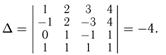
Because the

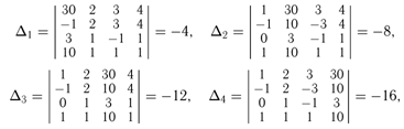
then, by virtue of Cramer’s formulas, the only solution to the system under consideration has the form x 1 = 1, x 2 = 2, x 3 = 3, x 4 = 4.
The main significance of Cramer's formulas is that they provide an explicit expression for solving a quadratic system of linear equations (with a nonzero determinant) in terms of the coefficients of the equations and the free terms. The practical use of Cramer's formulas involves rather cumbersome calculations (to solve a system of n equations with n unknowns, one has to calculate the (n + 1) nth-order determinant). To this it should be added that if the coefficients of the equations and free terms are only approximate values ​​of any measured physical quantities or are rounded during the calculation process, then the use of Cramer's formulas can lead to large errors and in some cases is inappropriate.
In §4 of Chapter 4, the regularization method due to A.N. will be presented. Tikhonov and allows one to find a solution to a linear system with an accuracy corresponding to the accuracy of specifying the matrix of equation coefficients and the column of free terms, and in Chap. 6 gives an idea of ​​the so-called iterative methods for solving linear systems, which make it possible to solve these systems using successive approximations of unknowns.
In conclusion, we note that in this section we excluded from consideration the case when the determinant Δ of the main matrix of system (3.10) vanishes. This case will be contained in general theory systems of m linear equations with n unknowns, presented in the next paragraph.
2. Finding all solutions of the general linear system. Let us now consider the general system of m linear equations with n unknowns (3.1). Let us assume that this system is consistent and that the rank of its main and extended matrices is equal to the number r. Without loss of generality, we can assume that the basis minor of the main matrix (3.2) is in the upper left corner of this matrix (the general case is reduced to this case by rearranging the equations and unknowns in the system (3.1).
Then the first r rows of both the main matrix (3.2) and the extended matrix (3.8) are the basis rows of these matrices (since the ranks of the main and extended matrices are both equal to r, the basis minor of the main matrix will simultaneously be the basis minor of the extended matrix) , and, by Theorem 1.6 on the basis minor, each of the rows of the extended matrix (1.8), starting from the (r + 1)th row, is a linear combination of the first r rows of this matrix.
In terms of system (3.1), this means that each of the equations of this system, starting with the (r + 1)th equation, is a linear combination (i.e., a consequence) of the first r equations of this system ( i.e., any solution of the first r equations of system (3.1) turns into identities all subsequent equations of this system).
Thus, it is sufficient to find all solutions of only the first r equations of system (3.1). Let us consider the first r equations of system (3.1), writing them in the form

If we give the unknowns x r+1 ,...,x n completely arbitrary values ​​c r+1 ,...,c n , then system (1.19) will turn into a quadratic system of r linear equations for r unknowns x 1 , x 2 , ..., x r , and the determinant of the main matrix of this system is the nonzero basis minor of matrix (3.2). Due to the results of the previous paragraph, this system (3.19) has a unique solution determined by Cramer’s formulas, i.e. for arbitrarily chosen c r+1 ,...,c n there is a unique collection of r numbers c 1 ,...,c r , turning all equations of system (3.19) into identities and defined by Cramer’s formulas.
To write down this unique solution, we agree to denote by the symbol M j (d i) the determinant obtained from the basis minor M of matrix (3.2) by replacing its j-ro column with a column of numbers d 1, d 2,...,d i,..., d r (with all other columns of M being preserved without changing). Then, writing the solution to system (3.19) using Cramer’s formulas and using the linear property of the determinant, we obtain

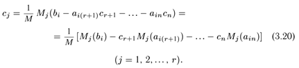
Formulas (3.20) express the values ​​of the unknowns x j = c j (j = 1, 2,......, r) through the coefficients of the unknowns, free terms and arbitrarily specified parameters with r+1,...., with n.
Let's prove that formulas (3.20) contain any solution to system (3.1). Indeed, let c (0) 1 , c (0) 2 ,...,c (0) r , c (0) r+1 , ...,c (0) n be an arbitrary solution of the specified system. Then it is a solution to system (3.19). But from system (3.19) the quantities c (0) 1 , c (0) 2 ,...,c (0) r are determined uniquely through the quantities c (0) r+1 , ...,c (0) n and precisely according to Cramer’s formulas (3.20). Thus, with r+1 = c (0) r+1 , ..., With n = c (0) n formulas (3.20) give us exactly the solution under consideration c (0) 1 , c (0) 2 ,...,c (0) r , c (0) r+1 , ...,c (0) n .
Comment. If the rank r of the main and extended matrices of system (3.1) is equal to the number of unknowns n, then in this case relations (3.20) turn into formulas

defining the unique solution of system (3.1). Thus, system (3.1) has a unique solution (i.e., it is definite) provided that the rank r of its main and extended matrices is equal to the number of unknowns n (and less than or equal to the number of equations m).
Example. Let's find all solutions of the linear system

It is easy to verify that the rank of both the main and extended matrices of this system is equal to two (i.e., this system is compatible), and we can assume that the basic minor M is in the upper left corner of the main matrix, i.e. . But then, discarding the last two equations and setting arbitrarily with 3 and with 4, we get the system

x 1 - x 2 = 4 - c 3 + c 4,

x 1 + x 2 = 8 - 2c 3 - 3c 4,

from which, by virtue of Cramer’s formulas, we obtain the values

x 1 = c 1 = 6 - 3/2 c 3 - c 4, x 2 = c 2 = 2 - 1/2 c 3 - 2c 4. (3.22)

So four numbers

(6 - 3/2 c 3 - c 4,2 - 1/2 c 3 - 2c 4,c 3, c 4) (3.23)

for arbitrarily given values ​​of c 3 and c 4 they form a solution to system (3.21), and line (3.23) contains all solutions of this system.

3. Properties of a set of solutions homogeneous system. Let us now consider a homogeneous system of m linear equations with n unknowns (3.7), assuming, as above, that the matrix (3.2) has rank equal to r, and that the basis minor M is located in the upper left corner of this matrix. Since this time all b i are equal to zero, instead of formulas (3.20) we get the following formulas:

expressing the values ​​of the unknowns x j = c j (j = 1, 2,..., r) through the coefficients of the unknowns and arbitrarily given values ​​c r+1 ,...,c n. Due to what was proven in the previous paragraph formulas (3.24) contain any solution of the homogeneous system (3.7).
Let us now make sure that the set of all solutions of the homogeneous system (3.7) forms a linear space.
Let X 1 = (x (1) 1, x (1) 2,...,x (1) n) and X 2 = (x (2) 1, x (2) 2,...,x ( 2) n) are two arbitrary solutions of the homogeneous system (3.7), and λ is any real number. Due to the fact that each solution of the homogeneous system (3.7) is an element of the linear space A n of all ordered collections of n numbers, it is sufficient to prove that each of the two collections

X 1 + X 2 = (x (1) 1 + x (2) 1 ,..., x (1) n + x (2) n)

λ X 1 = (λ x (1) 1 ,...,λ x (1) n)

is also a solution to the homogeneous system (3.7).
Let us consider any equation of system (3.7), for example the i-th equation, and substitute the elements of the indicated sets into this equation in place of the unknowns. Considering that X 1 and X 2 are solutions of a homogeneous system, we will have

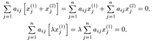
and this means that the sets X 1 + X 2 and λ X 1 are solutions to the homogeneous system (3.7).
So, the set of all solutions of the homogeneous system (3.7) forms a linear space, which we denote by the symbol R.
Let's find the dimension of this space R and construct a basis in it.
Let us prove that under the assumption that the rank of the matrix of the homogeneous system (3.7) is equal to r, the linear space R of all solutions of the homogeneous system (3.7) is isomorphic to the linear space A n-r all ordered collections of (n - r) numbers(the space A m was introduced in Example 3, Section 1, Section 1, Chapter 2).

Let us associate each solution (c 1 ,...,c r , c r+1 ,...,c n) of the homogeneous system (3.7) with an element (c r+1 ,...,c n) of the space A n-r Since the numbers c r+1 ,...,c n can be chosen arbitrarily and with each choice, using formulas (3.24), they uniquely determine the solution of system (3.7), then the correspondence we have established is one-to-one. Next, we note that if elements c (1) r+1 ,...,c (1) n and c (2) r+1 ,...,c (2) n of the space A n-r correspond to the elements (c (1) 1 ,...,c (1) r , c (1) r+1 ,...,c (1) n) and (c (2) 1 ,...,c (2) r , c (2) r+1 ,...,c (2) n) of the space R, then from formulas (3.24) it immediately follows that the element (c (1) r+1 + c (2 ) r+1 ,...,c (1) n +c (2) n) corresponds to the element (c (1) 1 + c (2) 1 ,...,c (1) r + c (2) r , c (1) r+1 + c (2) r+1 ,...,c (1) n +c (2) n), and the element (λ c (1) r+1 ,... ,λ c (1) n) for any real λ corresponds the element (λ c (1) 1 ,...,λ c (1) r , λ c (1) r+1 ,...,λ c (1 ) n). This proves that the correspondence we have established is an isomorphism.
Thus, the linear space R of all solutions of the homogeneous system (3.7) with n unknowns and the rank of the main matrix equal to r is isomorphic to the space A n-r and, therefore, has dimension n - r.
Any set of (n - r) linearly independent solutions of the homogeneous system (3.7) forms (by virtue of Theorem 2.5) a basis in the space R of all solutions and is called the fundamental set of solutions of the homogeneous system (3.7).
To construct a fundamental set of solutions, you can start from any basis in space A n-r. The set of solutions of system (3.7) corresponding to this basis, due to isomorphism, will be linearly independent and therefore will be a fundamental set of solutions.
Particular attention is paid to the fundamental set of solutions of system (3.7), which corresponds to the simplest basis e 1 = (1, 0, 0,..., 0), e 2 = (1, 1, 0,..., 0), ... , e n-r = (0, 0, 0,..., 1) spaces A n-r and called the normal fundamental set of solutions of the homogeneous system (3.7).
Under the assumptions made above about the rank and location of the basis minor, by virtue of formulas (3.24), the normal fundamental set of solutions of the homogeneous system (3.7) has the form:

By definition of the basis, any solution X of the homogeneous system (3.7) can be represented in the form

X= C 1 X 1 + C 2 X 2 + ... + C n-r X n-r , (3.26)

where C 1, C 2, ..., C n-r are some constants. Since formula (3.26) contains any solution to the homogeneous system (3.7), this formula gives the general solution to the homogeneous system under consideration.
Example. Consider a homogeneous system of equations:

corresponding to the inhomogeneous system (3.21), analyzed in the example at the end of the previous paragraph. There we found out that the rank r of the matrix of this system is equal to two, and we took the minor in the upper left corner of the specified matrix as the basis.
Repeating the reasoning carried out at the end of the previous paragraph, we obtain instead of formulas (3.22) the relations

c 1 = - 3/2 c 3 - c 4, c 2 = - 1/2 c 3 - 2c 4,

valid for arbitrarily chosen c 3 and c 4 . Using these relations (assuming first c 3 =1,c 4 =0, and then c 3 = 0,c 4 = 1) we obtain a normal fundamental set of two solutions to system (3.27):

X 1 = (-3/2,-1/2,1,0), X 2 = (-1,-2, 0.1). (3.28)

where C 1 and C 2 are arbitrary constants.
To conclude this section, we will establish a connection between the solutions of the inhomogeneous linear system (3.1) and the corresponding homogeneous system (3.7) (with the same coefficients for the unknowns). Let us prove the following two statements.
1°. The sum of any solution to the inhomogeneous system (3.1) with any solution to the corresponding homogeneous system (3.7) is a solution to system (3.1).
In fact, if c 1 ,...,c n is a solution to system (3.1), a d 1 ,...,d n is a solution to the corresponding homogeneous system (3.7), then, substituting in any (for example, in the i-th ) the equation of system (3.1) in place of the unknown numbers c 1 + d 1 ,...,c n + d n , we get

Q.E.D.
2°. The difference of two arbitrary solutions of the inhomogeneous system (3.1) is the solution of the corresponding homogeneous system (3.7).
In fact, if c" 1 ,...,c" n and c" 1 ,...,c" n are two arbitrary solutions of system (3.1), then, substituting in any (for example, in the i-th) equation of system (3.7) in place of the unknown numbers c" 1 - c" 1 ,...,c" n - c" n we get

Q.E.D.
From the proven statements it follows that, Having found one solution of the inhomogeneous system (3.1) and adding it with each solution of the corresponding homogeneous system (3.7), we obtain all solutions of the inhomogeneous system (3.1).
In other words, the sum of the particular solution of the inhomogeneous system (3.1) and the general solution of the corresponding homogeneous system (3.7) gives the general solution of the inhomogeneous system (3.1).
As a particular solution to the inhomogeneous system (3.1), it is natural to take that solution (it is assumed, as above, that the ranks of the main and extended matrices of the system (3.1) are equal to r and that the basic minor is in the upper left corner of these matrices)

which will be obtained if in formulas (3.20) we set all numbers c r+1 ,...,c n equal to zero. Adding this particular solution to the general solution (3.26) of the corresponding homogeneous system, we obtain the following expression for the general solution of the inhomogeneous system (3.1):

X= X 0 + C 1 X 1 + C 2 X 2 + ... + C n-r X n-r . (3.30)

In this expression, X 0 denotes a particular solution (3.29), C 1 , C 2 , ... , C n-r are arbitrary constants, and X 1 , X 2 ,... , X n-r are elements of the normal fundamental set of solutions (3.25) corresponding homogeneous system.
Thus, for the inhomogeneous system (3.21) considered at the end of the previous paragraph, a particular solution of the form (3.29) is equal to X 0 = (6,2,0, 0).
Adding this particular solution to the general solution (3.28) of the corresponding homogeneous system (3.27), we obtain the following general solution to the inhomogeneous system (3.21):

X = (6,2,0, 0) + C 1 (-3/2,-1/2,1,0) + C 2 (-1,-2, 0.1). (3.31)

Here C 1 and C 2 are arbitrary constants.
4. Concluding remarks on solving linear systems. Methods for solving linear systems developed in previous paragraphs
rests on the need to calculate the rank of the matrix and find its basis minor. Once the basis minor has been found, the solution comes down to the technique of calculating the determinants and the use of Cramer's formulas.
To calculate the rank of a matrix, you can use the following rule: when calculating the rank of a matrix, one should move from minors of lower orders to minors of higher orders; Moreover, if a non-zero minor M of order k has already been found, then only the minors of order (k + 1) bordering(that is, they contain the minor M inside themselves) this minor is M; if all bordering minors of order (k + 1) are equal to zero, the rank of the matrix is ​​equal to k(in fact, in the indicated case, all rows (columns) of the matrix belong to the linear hull of its k rows (columns), at the intersection of which there is a minor M, and the dimension of the indicated linear hull is equal to k).
Let us also indicate another rule for calculating the rank of a matrix. Note that with the rows (columns) of a matrix one can perform three elementary operations, which do not change the rank of this matrix: 1) permutation of two rows (or two columns), 2) multiplication of a row (or column) by any non-zero factor, 3) addition to one row (column) of an arbitrary linear combination of other rows (columns) (these three operations do not change the rank of the matrix due to the fact that operations 1) and 2) do not change the maximum number of linearly independent rows (columns) of the matrix, and operation 3) has the property that the linear span of all rows (columns) existing before performing this operation coincides with the linear envelope of all rows (columns) obtained after performing this operation).
We will say that the matrix ||a ij ||, containing m rows and n columns, has diagonal form, if all its elements other than a 11, a 22,.., a rr are equal to zero, where r = min(m, n). The rank of such a matrix is ​​obviously equal to r.
Let's make sure that using three elementary operations any matrix

can be reduced to diagonal form(which allows us to calculate its rank).

In fact, if all elements of matrix (3.31) are equal to zero, then this matrix has already been reduced to diagonal form. If the mother
ribs (3.31) have non-zero elements, then by rearranging two rows and two columns it is possible to ensure that the element a 11 is non-zero. After multiplying the first row of the matrix by a 11 -1, we will turn the element a 11 into one. Subtracting further from the j-ro column of the matrix (for j = 2, 3,..., n) the first column multiplied by a i1, and then subtracting from i-th line(for i = 2, 3,..., n) the first row multiplied by a i1, we get instead of (3.31) a matrix of the following form:

Performing the operations we have already described with a matrix taken in a frame, and continuing to act in a similar way, after a finite number of steps we will obtain a diagonal matrix.
The methods for solving linear systems outlined in the previous paragraphs, which ultimately use the apparatus of Cramer’s formulas, can lead to large errors in the case when the values ​​of the coefficients of the equations and free terms are given approximately or when these values ​​are rounded during the calculation process.
First of all, this applies to the case when the matrix corresponding to the main determinant (or basis minor) is poorly conditioned(i.e. when “small” changes in the elements of this matrix correspond to “large” changes in the elements of the inverse matrix). Naturally, in this case the solution to the linear system will be unstable(i.e., “small” changes in the values ​​of the coefficients of the equations and free terms will correspond to “large” changes in the solution).
The noted circumstances lead to the need to develop both other (different from Cramer’s formulas) theoretical algorithms for finding a solution, and numerical methods for solving linear systems.
In §4 chapter 4 we will get acquainted with regularization method by A.N. Tikhonova finding the so-called normal(i.e. closest to the origin) solution of the linear system.
Chapter 6 will provide basic information about the so-called iterative methods solutions of linear systems that allow solving these systems using successive approximations of unknowns.